BASIC ECONOMIC ORDER QUANTITY (EOQ) MODEL

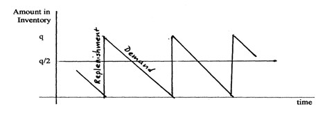
Look at the figure, which shows the number of units in inventory as a function of time.  The slanted lines show that items are being taken out of inventory as they are needed.  When the amount of inventory reaches zero, q units are ordered; they replenish the number of units in inventory to q.  Then, items are taken out of inventory, and the amount remaining declines again until it reaches zero.  Can you see why the average number of units in inventory is q/2?

     We want to minimize C(q), the total cost associated with having inventory if we order q units at a time.  The symbol "C(q)" means "C as a function of q," just like y = f(x) means "y is a function of x."  The Basic EOQ model seeks to find the optimal value of q--i.e., "q*"--that will minimize the total cost associated with having inventory.

               C(q) = A(q) + B(q) + D(q)

               where C(q) = total cost associated with the inventory if we order q units at a time
                         A(q) = holding cost
                         B(q) = shortage cost
                         D(q) = ordering cost

                    A(q) = C₁ • q/2

                    (i.e., "A of q" is equal to C₁ times q/2)

                    where C₁ = holding cost per unit of inventory

                    B(q) = 0

                    because "shortages are not allowed to occur" (this is an assumption of the Basic EOQ model)

                    D(q) = C₃ • r/q

                    where C₃ = cost of processing an order
                               r = total demand for a given period of time

                              r/q = number of orders

                    so          C(q) = A(q) + B(q) + D(q)

                                             = C₁ • q/2 + 0 + C₃ • r/q

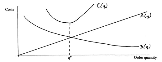
                    minimum C(q) occurs at q*

                         where A(q) and D(q) intersect

Because the minimum value of C(q)--i.e., C(q*)--occurs at the quantity q*, at which A(q*) = D(q*), we can use this information to solve for q*.

                         A(q*) = D(q*)

                         C₁ • q*/2 = C₃ • r/q*

Note:  In solving these problems, it is necessary that you use the same unit of time consistently.  Do not insert into the equation one variable that is in annual terms and another that is in monthly terms, for example.  Adjust the values of variables, as necessary, to express all of the variables in the same unit of time.

Problem #1:

Demand for pacemakers has been running at a rate of 10 per month. The cost of a pacemaker to the hospital is $1000. It costs $50 to place an order, and the hospital’s annual carrying cost is 12% of inventory value. Assuming the base EOQ model, what are q* and the minimum inventory cost?

Problem #2:

A small charter airline company wants to know how much aviation fuel to buy. Demand for flight fuel has been somewhat constant at 50,000 gallons per month. Fuel costs are 75 cents per gallon, and the company’s annual carrying-cost fraction is .10. It costs $100 to get a delivery with no lead time required.

1. What is the optimal order quantity?
2. What is the annual inventory cost resulting from ordering q*?

Problem #3:

An aerospace company has a contract with the U. S. Navy to produce 120 airplanes during the next year. The plan is to produce these airplanes at a rate of 10 per month. An actuating cylinder used to move the wing flap is purchased off the shelf from a nearby supplier; no lead time is required. Since there are two wings, two cylinders are needed per airplane. The actuating cylinders cost $200. Holding cost for the cylinders is $20 per year per cylinder. In addition, it costs $75 to order these cylinders and receive them from the vendor.

1. What is the optimal quantity?
2. What is the optimal number of orders per year?
3. What is the optimal time between orders?
4. What is the total inventory cost of ordering the optimal order quantity?