|
EVENTS THAT HAVE TAKEN AWAY THE POWER OF POLITICAL-PARTY
OFFICIALS
For many decades in American history, the political-party
organizations and their leaders had significant influence
over political campaigns, elections, and public policy.
However, events over the past 140 years have
drastically eroded the power of the political-party
organizations and their leaders.
Here is a discussion of these milestone events.
1.
Civil Service Act of 1883
After about half a century of experience with the “spoils
system” that President Andrew Jackson established when he
was elected in 1828, Americans decided that the spoils
system encouraged corruption in the national government.
The assassination of President James Garfield by a
so-called “disgruntled job seeker” was the final impetus for
Congress to enact the Civil Service of Act of 1883, whose
purpose was to begin the phasing-out of the spoils system
and the installation of the civil-service or “merit” system.
Jobs in the national government’s executive branch
below the policymaking level (i.e., below such positions as
Cabinet members, agency directors, and their immediate
subordinates) are covered by the civil service.
This includes a variety of professional jobs such as
agents, analysts, inspectors, accountants/bookkeepers,
scientists, engineers, etc.
It is a violation of the Civil Service Act of 1883
for appointments to those jobs to be determined based on
partisan affiliation.
The only acceptable criterion for appointment to the
civil service is merit.
This law eliminated influence by the party organizations and leaders in the
selection of executive-branch employees below the
policymaking level.
(At the policymaking level‑‑the highest levels in the
executive branch‑‑the appointments are “partisan
appointments” and the appointees are selected by the
president and his assistants.
The president is entirely entitled to take political
loyalty into consideration when he makes these partisan
appointments.)
2.
The “seniority system” was installed as a reform to break up
the speaker’s oligarchy (Joe Cannon vs. Champ Clark)
Up until 1910, the speaker of the U. S. House of
Representatives had enormous power over the
legislative/policymaking process.
He single-handedly decided who would be the chairmen
of the standing committees.
He also determined who would be the members of the
House Rules Committee, which determines which bills will
come to the House floor for debate and a vote.
The speaker worked closely with the chairman of his
party’s national committee and, together, they could decide
which policies would be established by law and which ones
would not. In
1910, there was an uprising against the last of the
all-powerful speakers‑‑Republican Joe Cannon‑‑led by Champ
Clark. Cannon
was ousted. The
members of the House took away the speaker’s unilateral
power to appoint the chairmen of the standing committees.
Thereinafter, on each standing committee, the
committee member who belonged to the majority party and had
the most seniority on the committee automatically became the
chairman. This
took enormous power away from the position of speaker and
from the position of the party’s national chairman, in so
far as they could not dictate policy anymore.
3.
The Hatch Act was enacted in 1939, prohibiting
national-government civil-service employees from openly
participating in politics
Even after the civil-service system had been installed to
reduce the power of the party organization and leadership
(so that they could not control appointments to
executive-branch positions as they did during the days of
the spoils system), suspicion persisted that, somehow, the
party leaders were still involved in placing loyal party members into government jobs
and that such loyal members were tithing their pay to the
political parties.
Therefore, to extinguish the link between the
political-party organizations and the civil service,
Congress enacted the Hatch Act of 1939.
This law prohibited civil servants from openly
participating in politics.
Thereinafter, they could not be a member of any
political organization or committee, they could not donate
to campaigns, they could not put yard signs in front of
their homes indicating their support for a candidate, etc.
4.
Primary elections for nominations took party leaders out of
the process (no more “smoke-filled rooms”)
In the 1910s, Robert La Follette of Wisconsin led the
Progressive Movement.
The centerpiece of the Progressive Movement’s beliefs
was a familiar one in American political history:
The movement’s
members were convinced that all of the corruption in
American politics originated in the political-party
organizations.
They demanded that the power to decide who the parties’
nominees for elected offices would be should be taken away
from the party leaders (who were denounced as “kingmakers”
who would make such decisions in “smoke-filled rooms”) and
transferred to the voters through the use of party primary
elections.
Journalists joined the Progressives’ demands that primary
elections become prevalent for selecting party nominees.
State by state, legislatures changed election laws to
require primary elections.
A principal influence of party leaders‑‑selection of
party nominees for elections‑‑was gradually eliminated
across the United States.
5.
U. S. Supreme Court:
Smith v. Allwright (1944) – “white primaries”
are illegal; parties are “inclusive”
In many of the racist, mostly southern, states, one of the
tricks used by the white, racist, elite class to
disfranchise black citizens was to declare the Democratic
state organizations to be private associations and to say
that, as private organizations, they possessed the right to
deny membership to black citizens.
Thus, the Democratic primaries in these states were
“white primaries.”
The nature of the abuse of this arrangement was based
on the Democrats’ monopoly of politics in the “Solid South”:
These states had banished the Republican party after
the Civil War to punish the party for prosecuting the war
against the southern states.
If Democratic voters could not vote in the Democratic
primaries, then, by the time that they
could vote in the general election, there was only one candidate
for each position:
the winner of the Democratic primary.
Thus, there was no way for black voters to have any
influence over who would get elected.
The U. S. Supreme Court accepted the case of
Smith v. Allwright,
321 U.S. 649 (1944).
In this case, the Supreme Court rejected the
Democratic state organizations’ claim to be private
associations; instead, the court said that these
organizations are unmistakably
public because of their influence in the process of elections.
The side-effect of the court’s opinion is that, since
then, the law has recognized that American political parties
are inclusive.
That means that anyone who wants to join either party
has the unqualified right to do so.
This characteristic of the political parties
decreases the party organizations’ and leaders’ power in
this regard: If
anyone who wants to be a member of either party is free to
do so, then the party leaders have very little ability to
impose discipline
on members.
Notably, the leaders lack the power to use
excommunication as
a form of discipline over disloyal individuals.
6.
Television allowed candidates to take their case directly to
the people
In the 1950s, many Americans purchased a new piece of
furniture for their living rooms:
television sets.
The development of television stations and networks
excited the political parties’ leaders:
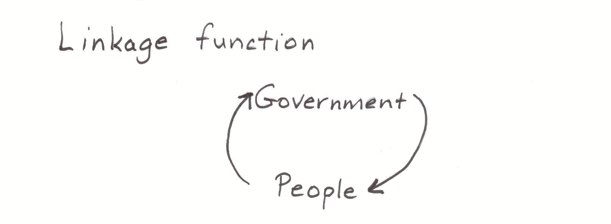
They anticipated that they could use the new medium
to carry out their
linkage function by sending messages over the airwaves
to the public to support the parties’ platforms and
candidates.
However, candidates had their own idea:
They could run their campaigns
independent of the
political-party organizations by appearing and advertising
on television!
Over time, it has become clear that the candidates’ vision
prevailed: The
vast majority of campaign advertisements are now made by and
paid for by candidates’
campaigns. “I’m
John Doe and I approve this message.”
Rare are campaign ads offered by, say, a Republican
State Central Committee advocating that voters should vote
for the Republican ticket in an upcoming statewide election.
7.
Members of Congress took over the “liaison” (ombudsman)
function
The ability of political-party leaders (e.g., local ward
chairmen and precinct captains) to deliver services to
individual party members has generally declined as
legislators have developed the function of
constituent service
(often known informally as “case work”).
Today, when a citizen is not getting a service from
the executive branch to which she believes she is entitled,
she does not contact a political-party leader.
Instead, she contacts the office of her U. S.
senator, U. S. representative, or state legislator,
depending on which level of government has the service to
which she feels entitled.
Legislators essentially stole this way of
ingratiating themselves with the public from the
political-party organizations.
8.
McGovern-Fraser Commission
In 1968, Democrats held a disastrous Democratic National
Convention in Chicago.
The delegates assembled there to nominate a candidate
for president.
Outside Chicago’s International Amphitheater, a variety of
anti-Vietnam War activists and civil-rights demonstrators
rioted in the streets.
The turmoil seeped into the arena, and the delegates
proceeded to demonstrate heated animosity toward each other.
The Democratic ticket led by Vice President Hubert H.
Humphrey went down to a painful defeat that November.
In the aftermath of this misfortune, the Democratic
National Committee appointed a Commission on Party Structure
and Delegate Selection.
The commission became popularly known as the
McGovern‑Fraser Commission, after the two members of
Congress who served as the chairmen at various times.
The commission focused on a deficiency of both
parties’ national conventions.
Those of us who would watch the conventions on
television would notice that the delegates were almost
uniformly older, affluent, white men.
These older,
affluent, white men, by the way, were almost all experienced
party leaders and their loyal supporters.
Thus, the commission developed rules that would
require state delegations at subsequent conventions to
properly represent women, black voters, Hispanics, laborers,
and young people.
The Democratic National Committee implemented the
commission’s recommendations.
When it was time for the 1972 Democratic convention
to convene, this time the delegates actually did include a
proportionate number of women, black voters, Hispanics,
laborers, and young people‑‑and, if the truth be told, they
were to a large extent
amateurs. A
lot of the older, affluent, white, male
party regulars‑‑many
of them members of Congress, state legislators, and other
experienced party activists‑‑were watching the convention on
television in their homes.
The amateurs bypassed former Vice President Humphrey,
who was making another attempt to become president, and
instead nominated U. S. Sen. George McGovern (D‑S. D.).
McGovern ran an anti-Vietnam War campaign during
which he presented the possibility that, as president, he
might pay a call on North Vietnamese Communist dictator Ho
Chi Minh and, on McGovern’s hands and knees, beg Ho for
peace. The
imagery troubled countless voters.
Republican incumbent Richard Nixon cleaned up the
floor with McGovern.
Causing the “party regulars” to stay at home and
allowing amateurs to make the final decision about the
Democratic nominee was just another insult for party leaders
and an indication of what happens when their power is taken
away.
Incidentally, to dampen the effect on the diversity rules
that excluded party regulars, the Democrats later added a
class of delegates known as “superdelegates”‑‑elected
government officials who would become delegates
automatically (i.e., without running in state presidential
primaries) and balance the diverse amateurs with their
experience.
Years, later, the presence of “superdelegates” would
complicate and inflame the bitter competition between
candidates Hillary Rodham Clinton and Bernie Sanders during
the 2016 contest for the Democratic nomination for
president.
Sanders’ supporters have been bitter about the effect of the
superdelegates, who overwhelmingly supported Clinton, ever
since.
9.
Nixon’s Committee to Reelect the President
President Nixon’s 1972 reelection campaign remains famous as
a milestone event because his campaign was
not run by the
Republican National Committee.
Instead, his campaign was run by his own candidate
committee, the “Committee to Reelect the President.”
The RNC’s chairman, Bob Dole, was irritated about
being bypassed in this manner, and referred to the committee
contemptuously as “CREEP.”
The committee ended up securing
another prominent
place in American history:
Operatives of the committee burglarized the
Democratic National Committee’s headquarters at the
Watergate hotel and office complex in Washington, D. C., as
they hoped to steal documents that would reveal the
Democrats’ campaign strategy.
The operatives were caught in the act and arrested.
A lengthy investigation followed.
Hoping to cover the operatives’ tracks, President
Nixon instructed his chief of staff and assistant for
domestic policy to direct the Federal Bureau of
Investigation to terminate its investigation to protect (nonexistent)
national-security secrets.
On account of obstructing justice by trying to
mislead the FBI, the president was forced to resign in
August 1974.
Arguably, he almost
ended up in a federal penitentiary, were he not pardoned by
his successor, Gerald Ford.
In fairness, it should be pointed out that Nixon’s decision
to entrust his reelection campaign to his own campaign
committee was not an irrational thing to do.
In modern times, thanks to such influences as La
Follette’s Progressive movement, political-party
organizations and leaders do
not decide who the
parties’ nominees will be.
Instead, every person who aspires to be elected has a
need, on her own, to secure the party’s nomination and‑‑to do so‑‑she
has to run against other aspirants in her party’s primary
election.
Obviously, the party organization is in no position to run
each such candidate’s primary campaign.
Each candidate must establish her own campaign
committee to help her win the primary.
Once one of the candidates has won the primary, is
she inclined to
dissolve her committee and turn her campaign over to the
party organization?
Of course not!
Her campaign committee has proved to be a winning
team.
Inevitably, she will rely on this committee to help her win
the general election.
10.
Transition committees
One might think that, when a candidate for president of the
United States has won the general election and he now has
about 3000 partisan appointments to make, he will call on
the chairman of his party’s national committee to help him
decide whom to appoint.
One who thinks that would be wrong.
In recent decades, the president-elect has
reorganized his campaign committee into a transition
committee, which will help the incoming president fill the
3000 positions.
The transition committee collects recommendations, résumés,
and other resources, and advises the new president how to
fill the partisan appointments.
The political-party organization is uninvolved in
this process, too.
11.
Open primaries
About half of the states have election laws that call for
“open primaries.”
Open primaries are the final insult to our
political-party organizations as policy-oriented
institutions.
Open-primary laws allow any voter‑‑regardless of any notion
of party affiliation‑‑to vote in either party’s primary on
primary-election day.
This allows, for example, unaffiliated voters
(“independents”) to vote in the Republican primary.
It even allows
Republicans to vote in the
Democratic
primary! The
original notion of political parties is that each political
party would present for the election a nominee who
represents the party’s policy-oriented mission.
Open primaries turn this notion into a joke.
They indicate just how much contempt our American
political system developed for the significance and
coherence of political parties.
The developments described above have certainly dispirited
political-party leaders.
Then-RNC chairman Bob Dole was trying at one point to
make an appointment with President Nixon.
He got as far as being able to discuss the matter in
a telephone call with Nixon’s chief of staff, H. R. “Bob”
Haldeman. Dole
later reported this only-somewhat-fictionalized dialogue:
DOLE: I'm the
national chairman and I need to see the president.
HALDEMAN: You
need to see the president?
Tune in Channel 9 tomorrow night at 10 o'clock.
An NGCSU political-science alumnus, Michael Shane McGonigal,
told me about how he was an intern in Washington, D. C., and
at a gala event he met Ken Mehlman, then Republican national
chairman. “Wow!”
Shane said.
“You’re the national chairman!
You are a powerful man!”
“Not really,” Mehlman replied.
“I’m just a glorified fund-raiser.”
|